Causal Inference Book Part I -- Glossary and Notes
June 19, 2019
This page contains some notes from Miguel Hernan and Jamie Robin’s Causal Inference Book. So far, I’ve only done Part I.
This page only has key terms and concepts. On this page, I’ve tried to systematically present all the DAGs in the same book. I imagine that one will be more useful going forward, at least for me.
Table of Contents:
- A few common variables
- Chapter 1: Definition of Causal Effect
- Chapter 2: Randomized Experiments
- Chapter 3: Observational Studies
- Chapter 4: Effect Modification
- Chapter 5: Interaction
- Chapter 6: Causal Diagrams
- Chapter 7: Confounding
- Chapter 8: Selection Bias
- Chapter 9: Measurement Bias
- Chapter 10: Random Variability
- Chapter 11: Why Model?
- Chapter 12:
A few common variables
| Variable | Meaning |
|---|---|
| A, E | Treatment |
| Y | Outcome |
| Y^(A=a) | Counterfactual outcome under treatment with \(a\) |
| Y^(a,e) | Joint counterfactual outcome under treatment with \(a\) and \(e\) |
| L | Patient variable (often confounder) |
| U | Patient variable (often unmeasured or background variable) |
| M | Patient variable (often effect modifier) |
Chapter 1: Definition of Causal Effect
| Term | Notation or Formula | Notes | Page |
|---|---|---|---|
| Association | Pr[Y=1|A=1] \(\neq\) Pr[Y=1|A=0] | Example definitions of independence (lack of association): Y \(\unicode{x2AEB}\) A or Pr[Y=1|A=1] - Pr[Y=1|A=0] = 0 or \(\frac{Pr[Y=1|A=1]}{Pr[Y=1|A=0]}\) = 1 or \(\frac{Pr[Y=1|A=1]/Pr[Y=0|A=1]}{Pr[Y=1|A=0]/Pr[Y=0|A=0]}\) = 1 |
I.10 |
| Causation and Causal Effects | Causation: Pr[Y^(a=1)=1] \(\neq\) Pr[Y^(a=0)=1] Individual Causal Effects: Y^(a=1) - Y^(a=0) Population Average Causal Effects: E[Y^(a=1)] - E[Y^(a=0)] where Y^(a=1) = Outcome for treatment w/ \(a=1\) Y^(a=0) = Outcome for treatment w/ \(a=0\) |
Sharp causal null hypothesis: Y^(a=1) = Y^(a=0) for all individuals in the population. Null hypothesis of no average causal effect: E[Y^(a=1)] = E[Y^(a=0)] Mathematical representations of causal null: Pr[Y^(a=1)=1] - Pr[Y^(a=0)=1] = 0 or \(\frac{Pr[Y^{a=1}=1]}{Pr[Y^{a=0}=1]} = 1\) or \(\frac{Pr[Y^{a=1}=1]/Pr[Y^{a=1}=0]}{Pr[Y^{a=0}=1]/Pr[Y^{a=1}=0]} = 1\) |
I.7 |
Chapter 2: Randomized Experiments
| Term | Notes | Page |
|---|---|---|
| Marginally randomized experiment | Single unconditional (marginal) randomization probability applied to assign treatments to all individuals in experiment. Produces exchangeability of treated and untreated. Values of counterfactual outcomes are missing completely at random (MCAR). |
I.18 |
| Conditionally randomized experiment | Randomized trial where study population is stratified by some variable \(L\), with different treatment probabilities for each stratum. Needn’t produce marginal exchangeability, but produces conditional exchangeability. Values of counterfactuals are not MCAR, but are missing at random (MAR) conditional on \(L\). |
I.18 |
| Standardization | Calculate the marginal counterfactual risk from a conditionally randomized experiment by taking a weighted average over the stratum-specific risks. Standardized mean: \(\sum_l E[Y|L=l,A=a] \times Pr[L=l]\) Causal risk ratio can be computed via standardization as follows: \(\frac{Pr[Y^{a=1}=1]}{Pr[Y^{a=0}=1]} = \frac{\sum_l E[Y=1|L=l,A=1]\times Pr[L=l]}{\sum_l E[Y=1|L=l,A=1]\times Pr[L=l]}\) |
I.19 |
| Inverse probability weighting | Given a conditionally randomized study population: 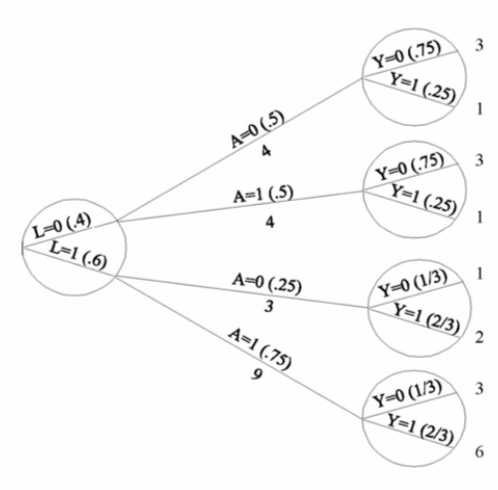 We can invoke an assumption of conditional exchangeability given \(L\) to simulate the counterfactual in which everyone had received (or not received) the treatment: 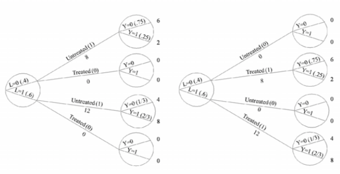 . The causal effect ratio can then be directly calculated by comparing \(Pr[Y^{a=1}=1]/Pr[Y^{a=0}=1]\) (in this example, it’s \(\frac{10/20}{10/20}=1\).) By the same token, you can effectively double your population and create a hypothetical pseudo-population in which everyone had received both treatments: 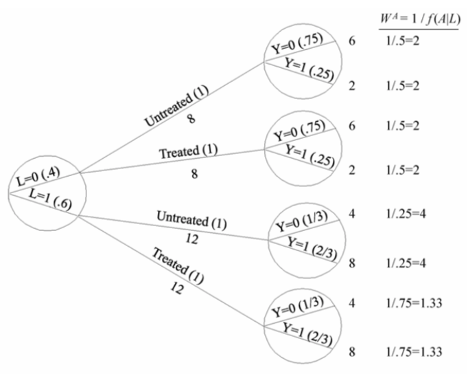 This process amounts to weighting each individual in the population by the inverse of the conditional probability of receiving the treatment she received (see formula on right above). Hence the name inverse probability (IP) weighting. |
I.20 |
Chapter 3: Observational Studies
| Term | Notation or Formula | English Definition | Notes | Page |
|---|---|---|---|---|
| Identifiability conditions | See below. | Sufficient conditions for conceptualizing an observational study as a randomized experiment. Consist of: 1. Consistency 2. Exchangeability, and 3. Positivity. |
I.25 | |
| Consistency | If \(A_i\) = \(a\), then \(Y_{i}^{a}=Y^{A_i}\) = \(Y_i\) | “The values of treatment under comparison correspond to well-defined interventions that, in turn, correspond to the versions of treatment in the data.” Has two main components: 1. Precise specification of counterfactual outcomes Y^a, and 2. Linkage of counterfactual outcomes to observed outcomes. |
Violated in an ill-defined intervention. Examples: - Study looks at “heart transplant” but doesn’t look at protocols (e.g. which immunosuppresant is used). If effect varies between versions of treatment and protocols not equally distributed, could cause problems. - Study wants to look at “obesity”, but “non-obesity” lumps together non-obesity from exercise vs cachexia vs genes vs diet. Need to subset population or make assumption that specific source of non-obesity doesn’t impact outcome. (Assumption called treatment-variation irrelevance assumption.) Not a testable assumption, relies on domain expertise. |
I.31 |
| Exchangeability (aka exogeneity) | Y^a \(\unicode{x2AEB}\) A for all \(a\) or Pr[Y^a=1 | A=1] = Pr[Y^a=1 | A=0] = Pr[Y^a=1] |
“The treated, had they remained untreated, would have experienced the same average outcome as the untreated did, and vice versa.” Essentially, this is the assumption of no unmeasured confounding. |
Beware formula: Not the same as Y \(\unicode{x2AEB}\) A, which would mean treatment has no effect on outcome. | I.27 |
| Conditional exchangeability | Y^a \(\unicode{x2AEB}\) A | L for all a or Pr[Y^a=1 | A=1, L=1] = Pr[Y^a=1 | A=0, L=1] = Pr[Y^a=1] | L=1 |
“The conditional probability of receiving every value of treatment is randomized or depends only on measured covariates” | Think conditional RCT where assigment depends only on \(L\). In observational studies, this is an untestable assumption, thus relies on domain expertise. |
I.27 |
| Positivity | Pr[A=a | L=\(l\) ] > 0 for all values \(l\) with Pr[L=\(l\)] \(\neq\) 0 in the population of interest | “The conditional probability of receiving every value of treatment is greater than zero, i.e. positive.” | Aka “Experimental treatment assumption” Example of positivity not holding: doctors always give heart transplants to patients in critical condition, eliminitating positivity from that stratum of an observational study. Unlike exchangeability, positivity, can be empricially verified. |
I.30 |
Chapter 4: Effect Modification
| Term | Notation or Formula | English Definition | Notes | Page |
|---|---|---|---|---|
| Effect modification aka effect-measure modification |
Additive effect modification: E[Y^(a=1)-Y^(a=0) | M = 1] \(\neq\) E[Y^(a=1)-Y^(a=0) | M = 0] Multiplicative effect modification: \(\frac{E[Y^{a=1} | M = 1]}{E[Y^{a=0} | M = 1]}\) \(\neq\) \(\frac{E[Y^{a=1}| M = 0]}{E[Y^{a=0}| M = 0]}\) |
\(M\) is a modifier of the effect of \(A\) on \(Y\) when the average causal effect of \(A\) on \(Y\) varies across levels of \(M\). | The null hypothesis of no average causal effect does not necessarily imply the absence of effect modification (e.g. equal and oppositive effect modifications in men and women could cancel at the population level), but the sharp null hypothesis of no causal effect does imply no effect modicifaction. We only count variables unaffected by treatment as effect modifiers. Similar variables that are effected by treatment are termed mediators. |
I.41 |
| Qualitative effect modification | Average causal effects in different subsets of the population go in opposite directions. | In presence of qualitative effect modification, additive effect modification implies multiplicative effect modification, and vice versa. In absence of qualitative effect modification, it’s possible to have only additive or only multiplicative effect modification. Effect modifiers are not necessarily assumed to play a causal role. To make this explicit, sometimes the terms surrogate effect modifier vs causal effect modifier are used, or you can play it even safer and refer to “effect heterogeneity across strata of \(M\).” Effect modification is helpful, among other things, for (i) assessing transportability to new populations where \(M\) may have different prevalences, (ii) choosing subpopulations that may most benefit from treatment, and (iii) identifying mechanisms leading to outcome if modifiers are mechanistically meaningful (e.g. circumscision for HIV transmission). |
I.42 | |
| Stratification | Statified causal risk differences: E[Y^(a=1) | M = 1] - E[Y^(a=0) | M = 1] and E[Y^(a=1) | M = 0] - E[Y^(a=0) | M = 0] |
To identify effect modification by variable \(M\), separately compute the causal effect of \(A\) on \(Y\) for each statum of the variable \(M\). | If study design assumes conditional rather than marginal exchangeability, analysis to estimate effect modification must account for all other variables \(L\) required to give exchangeability. This could involve standardization (IP weighting, etc.) by \(L\) within each stratum \(M\), or just using finer-grained stratification over all pairwise combinations of \(M\) and \(L\) (see page I.49). By the same token, stratification can be an alternative to standardization techinques such as IP weighting in analysis of any conditional randomized experiment : instead of estimating an average causal effect over the population while standardizing for \(L\), just stratify on \(L\) and report separate causal effect estimates for each stratum. |
I.43-49 |
| Collapsibility | A characteristic of a population effect measure. Means that the effect measure can be expressed as a weighted average of stratum-specific measures. | Examples of collapsible effect measures: risk ratio and risk difference Example of non-collapsible effect measure: odds ratio. Noncollapsibility can produce counter-intuitive findings like a causal odds ratio that’s smaller in the average population than in any stratum of the population. |
I.53 | |
| Matching | Construct a subset of the population in which all variables \(L\) have the same distribution in both the treated and the untreated. | Under assumption of conditional exchangeability given \(L\) in the source population, a matched population will have unconditional exchangeability. Usually, constructed by including all of the smaller group (e.g. the treated) and selecting one member of the larger group (e.g. the untreated) with matching \(L\) for each member in the smaller group. Often requires approximate matching. |
I.49 | |
| Interference | Treatment of one individual effects treatment status of other individuals in the population. | Example: A socially active individual convinces friends to join him while exercising. | I.48 | |
| Transportability | Ability to use causal effect estimation from one population in order to inform decisions in another (“target”) population. |
Requires that the target population is characterized by comparable patterns of: - Effect modification - Interference, and - Versions of treatment |
I.48 |
Chapter 5: Interaction
| Term | Notation or Formula | English Definition | Notes | Page |
|---|---|---|---|---|
| Joint counterfactual | Y^(a,e) | Counterfactual outcome that would have been observed if we had intervented to set the individual’s values of \(A\) (treatment component 1) to \(a\) and \(E\) (treatment component 2) to \(e\). | I.55 | |
| Interaction | Interaction on the additive scale: Pr[Y^(a=1,e=1)=1] - Pr[Y^(a=0,e=1)=1] \(\neq\) Pr[Y^(a=1,e=0)=1] - Pr[Y^(a=0,e=0)=1] or Pr[Y^(a=1) = 1 | E=1 ] - Pr[Y^(a=0) = 1 | E=1 ] \(\neq\) Pr[Y^(a=1) = 1 | E=0 ] - Pr[Y^(a=0) = 1 | E=0] |
The causal effect of \(A\) on \(Y\) after a joint intervention that set \(E\) to 1 differs from the causal effect of \(A\) on \(Y\) after a joint intervention that set \(E\) to 0. (Definition also holds if you swap \(A\) and \(E\).) | Different from effect modification because an effect modifier \(M\) is not considered a treatment or otherwise a variable on which we can intervene. In interaction, interventions \(A\) and \(E\) have equal status. Note from definition 2 on the left, however, that the mathematical definitions of effect modification and interaction line up. This means that if you randomize an interactor, it becomes equivalent to an effect modifier. Inference over joint counterfactuals require that the identifying conditions of exchangeability, positivity, and consistency hold for both treatments. |
I.55 |
| Counterfactual response type | A characteristic of an individual that refers to how she will respond to a treatment. | For example, an individual may have the same counterfactual outcome regardless of treatment, be helped by the treatment, or be hurt by the treatment. The presence of an interaction between \(A\) and \(E\) implies that some individuals exist such that their counterfactual outcomes under \(A=a\) cannot be determined without knowledge of \(E\). |
I.58 | |
| Sufficient-component causes | A set of variables that are sufficient to determine the outcome for a specific individual. | The minimal set of sufficient causes can be different for distinct ndividuals in the same study. For example, a patient with background factor \(U_1\) might have the same outcome regardless of treatment, whereas another patient’s outcome might be driven by both a treatment \(A\) and interactor \(E\). Minimal sufficient-component causes are sometimes visualized with pie charts. Contrast between counterfactual outcomes framework and sufficient-component-cause framework: Sufficient outcomes framework focuses on questions like: “given a particular effect, what are the various events which might have been its cause?” and counterfactual outcomes framework focuses on questions like: “what would have occurred if a particular factor were intervened upon and set to a different level than it was?”. Sufficient-component-causes requires more detailed mechanistic knoweldge and is generally more a pedagological tool than a data analysis tool. |
I.61 | |
| Sufficient cause interaction | A sufficient cause interaction between \(A\) and \(E\) exists in a population if \(A\) and \(E\) occur together in a sufficient cause. | Can be synergistic (A = 1 and E = 1 present in sufficient cause) or antagonistic (e.g. A = 1 and E = 0 is present in sufficient cause) . | I.64 |
Chapter 6: Causal Diagrams
| Term | Definition | Page |
|---|---|---|
| Path | A path on a DAG is a sequence of edges connecting two variables on the graph, with each edge occurring only once. | I.76 |
| Collider | A collider is a variable in which two arrowheads on a path collide. For example, \(Y\) is a collider in the path \(A \rightarrow Y \leftarrow L\) in the following DAG:  |
I.76 |
| Blocked path | A path on a DAG is blocked if and only if: 1. it contains a noncollider that has been conditioned, or 2. it contains a collider that has not been conditioned on and has no descendants that have been conditioned on. |
I.76 |
| d-separation | Two variables are d-separated if all paths between them are blocked | I.76 |
| d-connectedness | Two variables are d-connected if they are not d-separated | I.76 |
| Faithfulness | Faithulness is when all non-null associations implied by a causal diagram exist in the true causal DAG. Unfaithfulness can arise, for example, in certain settings of effect modification, by design as in matching experiments, or in the presence of certain deterministic relations between variables in the graph. | I.77 |
| Positivity (on graphs) | The arrows from the nodes \(L\) to the treatment node \(A\) are not deterministic. (Concerned with nodes into treatment nodes) | I.75 |
| Consistency (on graphs) | Well-defined intervention criteria: the arrow from treatment \(A\) to outcome \(Y\) corresponds to a potentially hypothetical but relatively unambiguous intervention. (Concerned with nodes leaving the treatment nodes.) | I.75 |
| Systematic bias | The data are insuffient to identify the causal effect even withan infinite sample size. This occurs when any sturctural association between treatment and outcome does not arise from the causal effect of treatment on outcome in the population of interest. | I.79 |
| Conditional bias | For average causal effects within levels of \(L\): Conditional bias exists whenever the effect measure (e.g. causal risk ratio) and the corresponding association measure (e.g. associational risk ratio) are not equal. Mathematically, this is when: \(Pr[Y^{a=1} | L = l] - Pr[Y^{a=0} | L = l]\) differs from \(Pr[Y|L=l, A = 1] - Pr[Y|L-l, A=0]\) for at least one stratum \(l\). For average causal effects in the entire population: Conditional bias exists whenever \(Pr[Y^{a=1} ] - Pr[Y^{a=0}]\) \(\neq\) \(Pr[Y = 1| A = 1] - Pr[Y = 1 | A = 0]\). |
I.79 |
| Bias under the null | When the null hypothesis of no causal effect of treatment on the outcome holds, but treatment and outcome are associated in the data. Can be from either confounding, selection bias, or measurement error.. |
I.79 |
| Confounding | The treatment and outcome share a common cause. | I.79 |
| Selection bias | Conditioning on common effects. | I.79 |
| Surrogate effect modifier | An effect modifier that does not dirrectly influence that outcome but might stand in for a causal effect modifier that does. | I.81 |
Chapter 7: Confounding
| Concept | Definition or Notes | Page |
|---|---|---|
| Backdoor Path | A noncausal path between treatment and outcome that remains even if all arrows pointing from treatment to other variables (the descendants of treatment) are removed. That is, the path has an arrow pointing into treatment. | I.83 |
| Confounding by indication (or Channeling) | A drug is more likely to be prescribed to individuals with a certain condition that is both an indication for treatment and a risk factor for the disease. | I.84 |
| Channeling | Confounding by indication in which patient-specific risk factors \(L\) encourage doctors to use certain drug \(A\) within a class of drugs. | I.84 |
| Backdoor Criterion | Assuming consistency and positivity, the backdoor criterion sets the circumstances under which (a) confounding can be eliminated from the analysis, and (b) a causal effect of treatment on outcome can be identified. Criterion is that identifiability exists if all backdoor paths can be blocked by conditioning on variables that are not affected by the treatment. The two settings in which this is possible are: 1. No common causes of treatment and outcome. 2. Common causes but enough measured variables to block all colliders. |
I.85 |
| Single-world intervention graphs (SWIG) | A causal diagram that unifies counterfactual and graphical approaches by explicitly including the counterfactual variables on the graph. Depicts variables and causal relations that would be observed in a hypothetical world in which all individuals received treatment level \(a\). In other words, is a graph that represents the counterfactual world created by a single intervention, unlike normal DAGs that represent variables and causal relations from the actual world. |
I.91 |
| Two categories of methods for confounding adjustment | G-Methods: G-formula, IP weighting, G-estimation. Exploit conditional exchangeability in subsets defined by \(L\) to estimate the causal effect of \(A\) on \(Y\) in the entire population or in any subset of the population. Stratification-based Methods: Stratification, Restriction, Matching. Methods that exploit conditional exchangeability in subsets defined by \(L\) to estimate the association between \(A\) and \(Y\) in those subsets only. |
I.93 |
| Difference-in-differences and negative outcome controls | A technique to account for unmeasured confounders under specific conditions. The idea is to measure a “negative outcome control”, which is the same as the main outcome but right before treatment. Then, instead of just reporting the effect of the treatment on the outcome (treatment effect + confounding effect), you substract out the effect of treatment on the negative outcome (only confounding effect). What’s left is is the difference-in-differences. This requires the assumption of additive equi-confounding: \(E[Y^{0}|A=1] - E[Y^{0}|A=0]\) = \(E[C|A=1] - E[C|A=0]\). Negative outcome controls are also sometimes used to try to detect confounding. Note: The DAG demonstration (Figure 7.11) is really useful for this one. |
I.95 |
| Frontdoor criterion and Frontdoor adjustment | A two-step standardization process to estimate a causal effect in the presence of a confounded causal effect that is mediated by an unconfounded mediator variable. Given a DAG such as:  \(Pr[Y^{a}=1] = \sum_{m}Pr[M^{a}=m]Pr[Y^{m}=1]\). Thus, standardization can be applied in two steps: 1. Compute \(Pr[M^{a}=m]\) as \(Pr[M=m| A=a]\), and 2. Compute \(Pr[Y^{a}=1]\) as \(\sum_{a'}Pr[Y=1|M=m,A=a']Pr[A=a']\) These are then combined with the formula \(\sum_{m}Pr[M=m| A=a]\sum_{a'}Pr[Y=1|M=m,A=a']Pr[A=a']\) The name frontdoor adjustment comes because it relies on the path from \(A\) and \(Y\) moving through a descendent \(M\) of \(A\) that causes \(Y\). |
I.96 |
Chapter 8: Selection Bias
Note: I have almost no notes in here, because the DAG section contains pretty much all the content I’m interested in noting here.
| Concept | Definition or Notes | Page |
|---|---|---|
| Competing Event | An event that prevents the outcome of interest from happening. For example, death is a competing event, because once it occurs, no other outcome is possible. | I.108 |
| Multiplicative survival model | A multiplicative survival model is of the form: \(Pr[Y=0|E=e,A=a]=g(e)h(a)\) . The data forllow such a model when there is no interaction between \(A\) and \(E\) on a multiplicative scale. This allows, for example, \(A\) and \(E\) to be conditionally independent given \(Y=0\) but not conditionally dependent when \(Y=1\). See Technical Point 8.2 and the example in Figure 8.13. |
I.109 |
| Healthy worker bias | Example of selection bias where people are only included in the study if they are healthy enough, say, to come into work and be tested. | I.99 |
| Self-selection bias | Example of selection bias where people volunteer for enrollment. | I.100 |
Chapter 9: Measurement Bias
| Concept | Definition or Notes | Page |
|---|---|---|
| Measurement bias or Information bias | Systematic difference in associational risk and causal risk that arises due to measurement error. Eliminates causal inference even under identifiability conditions of exchangeability, positivity, and consistency. | I.112 |
| __ Independent measurement error __ | Independent measurement error takes place when the measurement error of the treatment (\(U_{A}\)) and the measurement error of the response (\(U_{Y}\)) are d-separated. Dependent measurement error is when they are d-connected. | I.11 |
| __ Nondifferential measurement error __ | Measurement error is nondifferential with respect to the outcome if \(U_{A}\) and \(Y\) are d-separated. Measurement error is nondifferential with respect to the treatment if \(U_{Y}\) and \(A\) are d-separated. | I.11 |
| Intention-to-treat effect | The causal effect of randomized treatment assigment \(Z\) in an intention-to-treat trial on the outcome \(Y\). Depends on the strength of the effect of assignment treatment on outcome (\(Z \rightarrow Y\)), the assignment treatment on actual treatment received (\(Z \rightarrow A\)), and the effect of the actual treatment received on outcome (\(A \rightarrow Y\)). In theory, this does not require adjustment for confounding, has null preservation, and is conservative. See below for comments on latter two. | I.116 |
| The exclusion restriction | (The goal of double-blinding). The assumption that there is no direct arrow from assigned treatment \(Z\) to outcome \(Y\) in an intention-to-treat design. | I.117 |
| Null Preservation in an IIT | If treatment \(A\) has a null effect on \(Y\), then assigned treatment \(Z\) also has a null effect on \(Y\). Ensure, in theory, that a null effect will be declared when none exists. However, it requires that the exclusion restriction holds, which breaks down unless their is perfect double-blinding. | I.119 |
| Conservatism of the IIT vs Per-protocol | The IIT effect is supposed to be closer to the null than the value of the per-protocol effect, because imperfect adherence results in attenuation rather than exaggeration of effect. Thus IIT appears to be a lower bound for per-protocol effect (and is thus conservative). However, there are three issues with this: 1. Argument assumes monotonicity of effects (treatment same direction for all patients). If, say, there is inconsistent adherence and thus inconsistent effects, then this could become anti-conservative. 2. Even given monotonicity, IIT would only be conservative compared to placebos, not necessarily head-to-head trials, where adherence in the second drug might be different. 3. Even if IIT is conservative, this makes it dangerous when goal is evaluating safety, where you arguably want to be more aggresive in finding signal. |
|
| Per-protocol effect | The causal effect of randomized treatment that would have been observed if all individuals had adhered to their assigned treatment as specified in the protocol of the experiment. Requires adjustment for confounding. | I.116 |
| As-treated analysis | An analysis to assess for per-protocol effect. Includes all patients and compares those treated (\(A=1\)) vs not treated (\(A=0\)), independent of their assignment \(Z\). Confounded. | I.118 |
| Conventional per-protocol analysis | An analysis to assess for per-protocol effect. Limits the population to those who adhered to the study protocol, subsetting to those for whom \(A=Z\). Induces a selection bias on \(A=Z\), and thus still requires adjustment on \(L\). | I.118 |
| Tradeoff between ITT and Per-protocol | Summary: Estimating the per-protocol effect adds unmeasured confounding, which needs to be (imperfectly) adjusted for. Intention-to-treat adds a misclassification bias, and does not necessarily deliver on purported guarantees of conservatism. As such, there is a real tradeoff, here. | I.117-I.120 |
Chapter 10: Random Variability
Sorry, I’m skipping this section, because the key terms are all stats concepts and its mostly a pump-up chapter for the rest of the book.
Chapter 11: Why Model?
| Concept | Definition or Notes | Page | |
|---|---|---|---|
| Saturated Models | Models that do not impose restrctions on the data distribution. Generally, these are models whose number of parameters in a conditional mean model is equal to the number of means. For example, a linear model E[ y | x] ~ b0 + b1*x when the population is stratified into only two groups. These are non-parametric models. | II.143 |
| Non-parametric estimator | Estimators that produce estimates from the data without any a priori restrictions on the true function. When using the entire population rather than a sample, these yield the true value of the population parameter. | II.143 |
Chapter 12:
| Concept | Definition or Notes | Page |
|---|---|---|
| Stabilized Weights | ||
| Marginal Structure Model |
To-do: | Concept | Formula | Code | Notes | | :———–: |:————-:| | IP Weighting | | | | Standardized IP Weighting | | | | Marginal Structure model | | |
DONT MISS THE DOUBLY ROBUST ESTIMATOR in TECHNICAL POINT 13.2