All the DAGs from Hernan and Robins' Causal Inference Book

June 19, 2019

This is my preliminary attempt to organize and present all the DAGs from Miguel Hernan and Jamie Robin’s excellent Causal Inference Book. So far, I’ve only done Part I.

I love the Causal Inference book, but sometimes I find it easy to lose track of the variables when I read it. Having the variables right alongside the DAG makes it easier for me to remember what’s going on, especially when the book refers back to a DAG from a previous chapter and I don’t want to dig back through the text. Plus, making this was a great exercise!

Again, this page is meant to be fairly raw and only contain the DAGs. If you use it, you might also find it useful to open up this page, which is where I have more traditional notes covering the main concepts from the book. But of course, the text itself has no substitute.

Table of Contents:

Refresher: Visual rules of d-separation.
Refresher: Backdoor criterion
Basics of Causal Diagrams (6.1-6.5)
Effect Modification (6.6)
Confounding (Chapter 7)
Selection Bias (Chapter 8)
Measurement Bias (Chapter 9)

Refresher: Visual rules of d-separation.

Two variables on a DAG are d-separated if all paths between them are blocked. The following four rules defined what it means to be “blocked.”

(This is just meant to be a refresher – see the second half of this post or Fine Point 6.1 of the text for more definitions.)

Rule	Example
1. If there are no variables being conditioned on, a path is blocked if and only if two arrowheads on the path collide at some variable on the path.	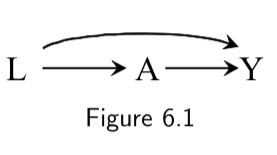\(L \rightarrow A \rightarrow Y\) is open. \(A \rightarrow Y \leftarrow L\) is blocked at \(Y\)
2. Any path that contains a noncollider that has been conditioned on is blocked.	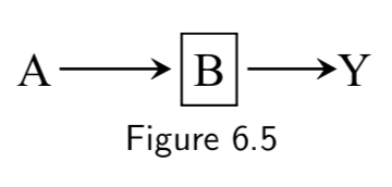Conditioning on \(B\) blocks the path from \(A\) to \(Y\).
3. A collider that has been conditioned on does not block a path	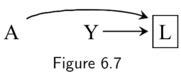The path between \(A\) and \(Y\) is open after conditioning on \(L\).
4. A collider that has a descendant that has been conditioned on does not block a path.	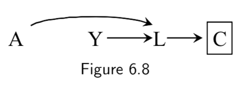The path between \(A\) and \(Y\) is open after conditioning on \(C\), a descendant of collider \(L\).

Refresher: Backdoor criterion

Assuming positivity and consistency, confounding can be eliminated and causal effects are identifiable in the following two settings:

Rule	Example
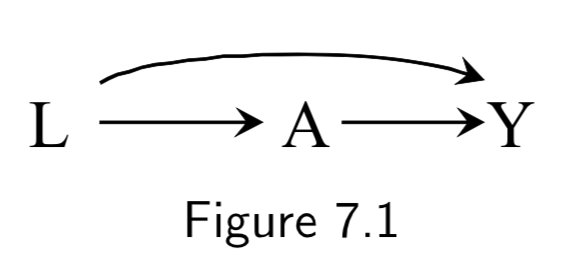
1. No common causes of treatment and outcome.	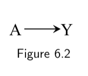There are no common causes of treatment and outcome. Hence no backdoor paths need to be blocked. No confounding; equivalent to a marginally randomized trial.
2. Common causes are present, but there are enough measured variables to block all colliders. (i.e. No unmeasured confounding.)	Backdoor path through the common cause \(L\) can be blocked by conditioning on measured covariates (in this case, \(L\) itself) that are non-descendants of treatment. There will be no residual confounding after controlling for \(L\); equivalent to a conditionally randomized trial.

And now we can finally:

Basics of Causal Diagrams (6.1-6.5)

DAG	Example	Notes	Page
	Marginally randomized experiment A: Treatment Y: Outcome	Arrow doesn’t specifically imply protection vs risk, just causal effect. Unconditional exchangeability assumption means that association implies causation and vice versa.	I.70
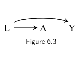
	Conditionally randomized experiment L: Stratification Variable A: Treatment Y: Outcome	Also equivalent to an Observational Study that assumes A depends on L and on no other causes of Y (else they’d need to be added). Implies conditional exchangeability.	I.69-I.70
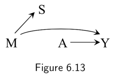
	A: Aspirin B: Platelet aggregation Y: Heart Disease	\(B\) is a mediator of \(A\)’s effect on \(Y\), but conditioning on \(B\) (e.g by restricting the analysis to people with a specific lab value) blocks the flow of association through the path A \(\rightarrow\) B \(\rightarrow\) Y. Even though \(A\) and \(Y\) are marginally associated, they are conditionally independent given \(B\). In other words, A \(\unicode{x2AEB}\) Y \| B. Thus, knowing aspirin status gives you no more information once platelets are measured, at least according to this graph.	I.73
	L: Smoking status A: Carrying a lighter Y: Lung cancer	Graph says that carrying a lighter (A) has no causal effect on outcome (Y). Math form of this assumption is: Pr[Y^(a=1)=1]=Pr[Y^(a=0)=1] However, \(A\) will be spuriously associated with \(Y\), because path A \(\leftarrow\) L \(\rightarrow\) Y is open to flow from A to Y: they share a common cause.	I.72
	L: Smoking status A: Carrying a lighter Y: Lung cancer	A \(\unicode{x2AEB}\) Y \| L, because the path A \(\leftarrow\) L \(\rightarrow\) Y is closed by conditioning on L. Thus, restricting the analysis to either smokers or non-smokers (box around L) means that lighter carrying will no longer be associated with lung cancer.	I.74
	A: Genetic predisposition for heart disease Y: Smoking status L: Heart disease	\(A\) and \(Y\) are not marginally associated, because they share no common causes. (i.e. Genetic risk for heart disease says nothing, in a vaccuum, about smoking status.) \(L\) here is a collider on the path A \(\rightarrow\) L \(\leftarrow\) Y, because the two arrows collide on this node. But there is no causal path from \(A\) to \(Y\).	I.73
	A: Genetic predisposition for heart disease Y: Smoking status L: Heart disease	Conditioning on the collider \(L\) opens the causal path A \(\rightarrow\) L \(\leftarrow\) Y. Put another way, two causes of a given effect generally become associated once we stratify on the common effect. In the example, knowing someone with heart disease lacks haplotype A makes it more likely that the individual is a smoker, because, in the absence of \(A\), it is more likely that some other cause of \(L\) is present. Or, conversely, the population of non-smokers with heart disease will be enriched for people with haplotype A. Thus, if one restricts the analysis to people with heart disease, he will find a spurious anti-correlation between the haplotype predictive of heart disease and smoking status.	I.74
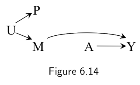
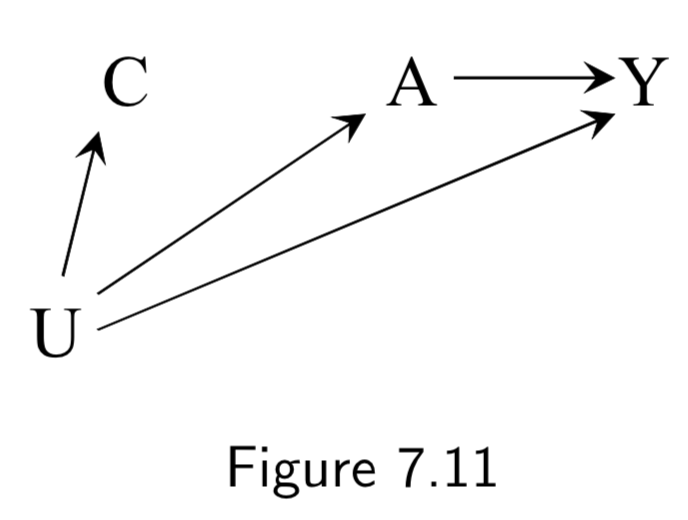
	A: Genetic predisposition for heart disease Y: Smoking status L: Heart disease C: Diuretic medication (given after heart disease diagnosis)	Conditioning on variable \(C\) downstream from collider \(L\) also opens up causal path A \(\rightarrow\) L \(\leftarrow\) Y. Thus, in the example, stratifying on \(C\) (diuretic status) will induce a spurious relationship between \(A\) (genetic heart disease risk) and \(Y\) (smoking status).	I.75
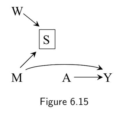
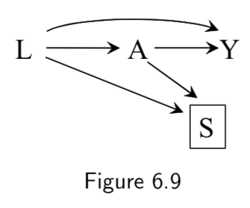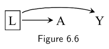
Before matching: After matching:	Matched analysis L: Critical Condition A: Heart Transplant Y: Death S: Selection for inclusion via matching criteria	In this study design, the average causal effect of \(A\) on \(Y\) is computed after matching on \(L\). Before matching, \(L\) and \(A\) are associated via the path \(L \rightarrow A\) . Matching is represented in the DAG through the addition of \(S\), the selection criteria. The study is obviously restricted to patients that are selected (\(S\)=1), hence we condition on \(S\). d-separation rules say that there are now two open paths between \(A\) and \(L\) after conditioning on \(S\): \(L \rightarrow A\) and \(L \rightarrow S \leftarrow A\). This seems to indicate an association between \(L\) and \(A\). However, the point of matching is supposed to be to make sure that \(L\) and \(A\) not associated! The resolution comes from the observation that \(S\) has been constructed specifically to induce the distribution of \(L\) to be the same in the treated (\(A\)=1) and untreated (\(A\)=0) population. This means that the association in \(L \rightarrow S \leftarrow A\) is of equal magnitude but opposite direction of \(L \rightarrow A\). Thus there is no net association between \(A\) and \(L\). This disconnect between the associations visible in the DAG and the associations actually present is an example of unfaithfulness, but here it has been introduced by design.	I.49 and I.79
	R: Compound treatment (see right) A: Vector of treatment versions \(A( r )\) (see right) Y: Outcome L and W: unnamed causes U: unnmeasured variables	This is the example the book uses of how to encode compound treatments. The example compound treatment is as follows: R=0 corresponds to “exercising less than 30 minutes daily”. R=1 corresponds to “exercising more than 30 minutes daily.” \(A\) is a vector corresponding to different versions of the treatment, where \(A(r=0)\) can take on values \(0,1,2,\dots, 29\) and \(A(r=1)\) can take on values \(30,31\dots, max\) Taken together, we can have a mapping from multiple values \(A( r )\) onto a single value \(R=r\).	I.78

Effect Modification (6.6)

Example	Notes	Page
A: Heart Transplant Y: Outcome M: Quality of Care. High (\(M=1\)) vs Low (\(M=0\))	This DAG reflects the assumption that quality of care influences quality of transplant procedure and thus of outcomes, BUT still assumes random assignment of treatment. Given random assignment, \(M\) is not strictly necessary but added if you want to use it to stratify. Causal diagram as such does not distinguish between: 1. Causal effect of treatment \(A\) on mortality \(Y\) is in the same direction in both stratum \(M=1\) and \(M=0\). 2. The causal effect of \(A\) on \(Y\) is in the opposite direction in \(M=1\) vs \(M=0\). 3. Treatment \(A\) as a causal effect on \(Y\) in one straum of \(M\) but no effect in other stratum.	I.80
A: Heart Transplant Y: Outcome M: Quality of Care. High (\(M=1\)) vs Low (\(M=0\)) N: Therapy Complications	Same example as above, except assumes that other variables along the path of a modifier can also influence outcomes.	I.80
A: Heart Transplant Y: Outcome M: Quality of Care. High (\(M=1\)) vs Low (\(M=0\)) S: Cost of treatment	Same example as above, except assumes that the quality of care effects the cost, but that the cost does not influence the outcome. This is the example of an effect modifier that does not have a causal effect on the outcome, but rather stands as a surrogate effect modifier. Analysis stratifying on \(S\) – which is available/objective – might be used to detect effect modification that actually comes from \(M\) but is harder to measure.	I.80
A: Heart Transplant Y: Outcome M: Quality of Care. High (\(M=1\)) vs Low (\(M=0\)) U: Place of residence P: Passport-defined nationality	Example where the surrogate effect modifier (passport) is not driven by the causal effect modifier (quality of care), but rather both are driven by a common cause (place of residence).	I.80
A: Heart Transplant Y: Outcome M: Quality of Care. High (\(M=1\)) vs Low (\(M=0\)) S: Cost of Care W: Use of mineral water vs tap	Example where the surrogate effect modifier (cost) is influenced by both the causal effect modifier (quality) and something spurious. If the study were restricted to low-cost hospitals by conditioning on \(S=0\), then use of mineral water would become associated with medical care \(M\) and would behave as a surrogate effect modifier. Addendum: How? One example might be that conditioned on a low cost, a zero sum situation may arise in which spending more on fancy water means less is being spent on quality care, which could yield an inverse correlation between mineral water and medical quality.	I.81

Confounding (Chapter 7)

DAG	Example	Notes	Page
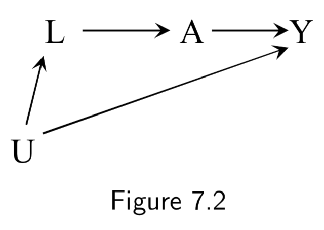
	L: Being physicially fit A: Working as a firefighter Y: Mortality	The path \(A \rightarrow Y\) is a causal path from \(A\) to \(Y\). \(A \leftarrow L \rightarrow Y\) is a backdoor path between \(A\) and \(Y\), mediated by common cause (confounder) \(L\). Conditioning on \(L\) will block the backdoor path, induce conditional exchangeability, and allow for causal inference. Note: This is an example of “healthy worker bias.”	I.83
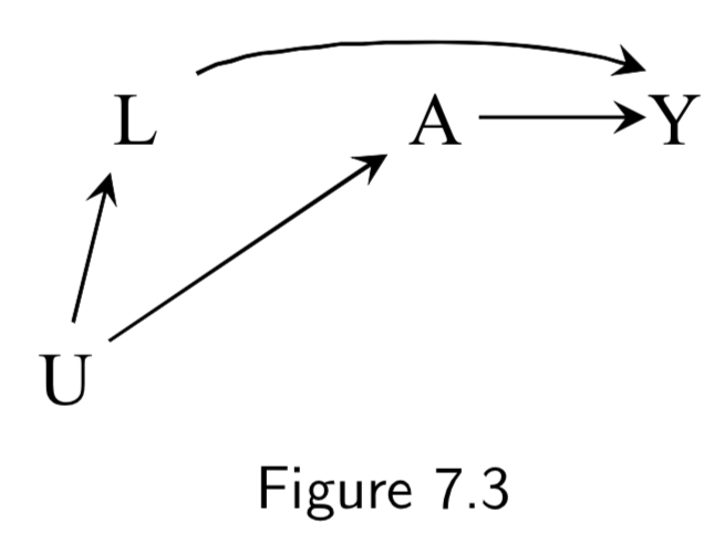
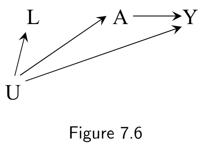
	A: Aspirin Y: Stroke L: Heart Disease U: Atherosclerosis (unmeasured)	This DAG is an example of confounding by indication (or channeling). Aspirin will have a confounded association with stroke, both from heart disease (\(L \rightarrow A \rightarrow Y\)), and from atherosclerosis (\(U \rightarrow L \rightarrow A \rightarrow Y\)). Conditioning on unmeasured \(U\) is impossible, but there is no unmeasured confounding given \(L\), so conditioning on \(L\) is sufficient.	I.84
	A: Exercise Y: Death L: Smoking status U: Social Factors (unmeasured) or Sublinical Disease (undetected)	Conditioning on \(L\) is again sufficient to block the backdoor path in this case.	I.84
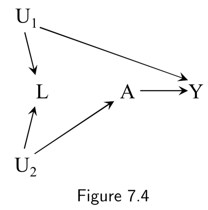	A: Physical activity Y: Cervical Cancer L: Pap smear U_1: Pre-cancer lesion (unmeasured here) U_2: Health-conscious personality (unmeasured)	Example shows how conditioning on a collider can induce bias. Adjustment for \(L\) (e.g. by restricting to negative tests \(L=0\)) will induce bias by opening a backdoor path between \(A\) and \(Y\) (\(A \leftarrow U_2 \rightarrow L \leftarrow U_1 \rightarrow Y\)), previously blocked by the collider. This is a case of selection bias. Thus, after conditioning, association between \(A\) and \(Y\) would be a mixture of association due to effect of \(A\) on \(Y\) and backdoor path. In other words, there is no unconditional bias, but there would be a conditional bias for at least one stratum of \(L\).	I.88
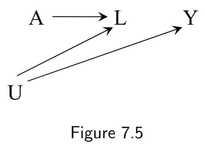	(Labels not in book) A: Antacid L: Heartburn Y: Heart attack U: Obesity	A nonconfounding example in which traditional analysis might lead you to adjust for \(L\), but doing so would induce a bias.	I.89
	A: Physical activity L: Income Y: Cardiovascular disease U: Socioeconomic status	\(L\) (income) is not a confounder, but is a measurable variable that could serve as a surrogate confounder for \(U\) (socioeconomic status) and thus could be used to partially adjust for the confounding from \(U\). In other words, conditioning on \(L\) will result in a partial blockage of the backdoor path \(A \leftarrow U \rightarrow Y\).	I.90
Normal DAG: Corresponding SWIG:	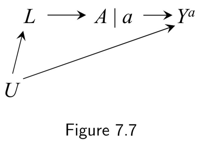A: Aspirin Y: Stroke L: Heart Disease U: Atherosclerosis (unmeasured)	Represents data from a hypothetical intervention in which all individuals receive the same treatment level \(a\). Treatment is split into two sides: (a) Left side encodes the values of treatment \(A\) that would have been observed in the absence of intervention (the natural value of treatment) (b) Right side encodes the treatment value under the intervention. \(A\) has no variable into \(a\) bc \(a\) is the same everywhere. Conditional exchangeability \(Y^{a} \unicode{x2AEB} A \| L\) holds because all paths between \(Y^{a}\) and \(A\) are blocked after conditioning on \(L\).	I.91
Normal DAG: Corresponding SWIG:	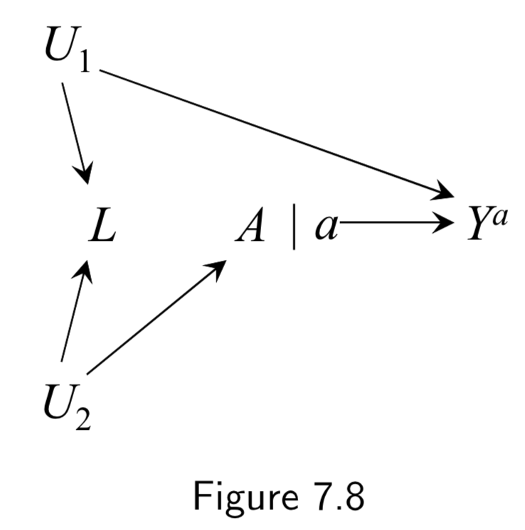A: Physical activity Y: Cervical Cancer L: Pap smear U_1: Pre-cancer lesion (unmeasured here) U_2: Health-conscious personality (unmeasured)	Here, marginal exchangeability \(Y^{a} \unicode{x2AEB} A\) holds because, on the SWIG, all paths between \(Y^{a}\) and \(A\) are blocked without conditioning on \(L\). Conditional exchangeability \(Y^{a} \unicode{x2AEB} A \| L\) does not hold because, on the SWIG, the path \(Y^{a} \leftarrow U_1 \rightarrow L \leftarrow U_2 \rightarrow A\) is open when the collider \(L\) is conditioned on. Taken together, marginal \(A-Y\) association is causal but conidtional association \(A-Y\) given \(L\) is not.	I.91
Normal DAG: 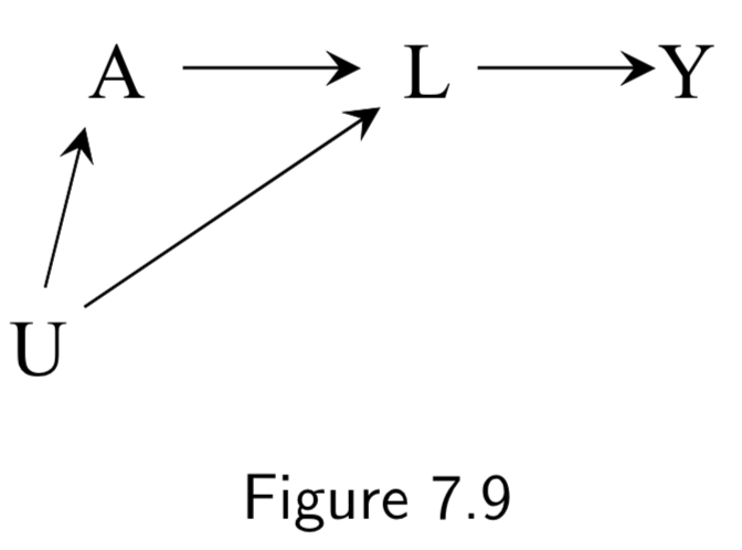Corresponding SWIG:	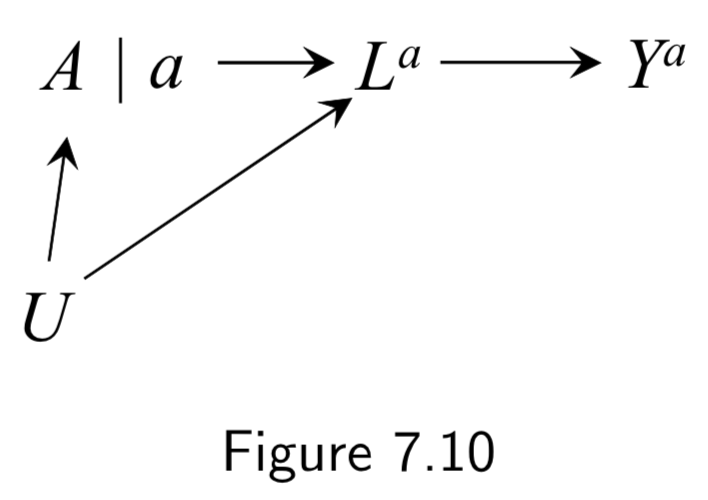(Example labels not in book) A: Statins Y: Coronary artery disease L: HDL/LDL U: Race	In this example, the SWIG is used to highlight a failure of the DAG to provide conditional exchangeability \(Y^{a} \unicode{x2AEB} A \| L\). In the SWIG, the factual variable \(L\) is replaced by the counterfactual variable \(L^{a}\). In this SWIG, counterfactual exchangeability \(Y^{a} \unicode{x2AEB} A \| L_{a}\) holds, since \(L^{a}\) blocks the paths from \(Y^{a}\) to \(A\). But \(L\) is not even on the graph, so we can’t conclude \(Y^{a} \unicode{x2AEB} A \| L\) holds. The problem being highlighted here is that \(L\) is a descendent of the treatment \(A\) blocking the path to \(Y\). In contrast, if the arrow from \(A\) to \(L\) didn’t exist, \(L\) would not be a descendent of \(A\) and adjusting for \(L\) would eliminate all bias, even if \(L\) were still in the future of \(A\). Thus, confounders are allowed to be in the future of the treatment, they just can’t be descendents.	I.92
	A: Aspirin Y: Blood Pressure U: History of heart disease (unmeasured) C: Blood pressure right before treatment (“placebo test” aka “negative outcome control”)	This example was used to show difference-in-difference and negative outcome controls. The idea: We cannot compute the effect of \(A\) on \(Y\) via standardization or IP weighting because there is unmeasured confounding. Instead, we first measure the (“negative”) outcome \(C\) right before treatment. Obviously \(A\) has no effect on \(C\), but we can assume that \(U\) will have the same confounding effect on \(C\) that it has on \(Y\). As such, we take the effect in the treated to be the effect of \(A\) on \(Y\) (treatment effect + confounding effect) minus the effect of \(A\) on \(C\) (confounding effect). This is the difference-in-differences. Negative outcome controls are sometimes used to try to detect confounding.	I.95
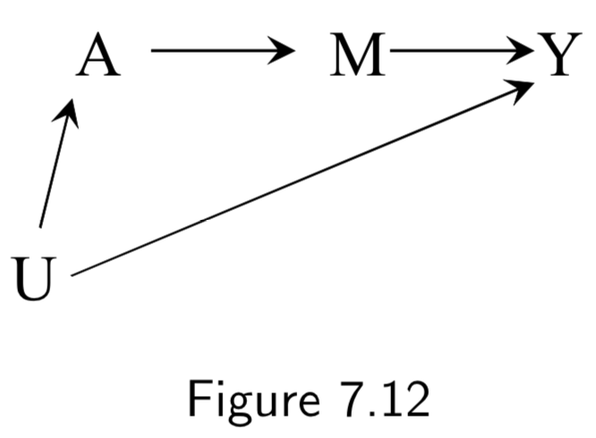	(No example labels in text) A: Aspirin M: Platelet Aggregation Y: Heart Attack U: High Cardiovascular Risk	This example is to demonstrate the frontdoor criterion (see notes or page I.96 for more details). Given this DAG, it is impossible to directly use standardization or IP weighting, because the unmeasured variable \(U\) is necessary to block the backdoor path between \(A\) and \(Y\). However, the frontdoor adjustment can be used because: (i) the effect of \(A\) on \(<\) can be computed without confounding, and (ii) the effect of \(M\) on \(Y\) can be computed because \(A\) blocks only the backdoor path. Hence, frontdoor adjustment can be used.	I.95

Some additional (but structurally redundant) examples of confounding from chapter 7:

Example	Notes	Page
A: Exercise Y: Death L: Smoking status U: Social Factors (unmeasured) or Sublinical Disease (undetected)	Subclinical disease could also result both in lack of exercise \(A\) and increased risk of a clinical diseae \(Y\). This is an example of reverse causation.	I.84
A: Gene being tested Y: Trait L: Different gene in LD with gene A U: Ethnicity	Linkage disequilibrium can drive spurious associations between gene \(A\) and trait \(Y\) if the true causal gene \(L\) is in LD with \(A\) in patients with ethnicity \(U\).	I.84
A: Airborne particulate matter Y: Coronary artery disease L: Other pollutants U: Weather conditions	Environmental exposures often co-vary with the weather conditions. As such, certain pollutants \(A\) may be spuriously associated with outcome \(Y\) simply because the weather drives them to co-occur with \(L\).	I.84

Selection Bias (Chapter 8)

Note: While randomization eliminates confounding, it does not eliminate selection bias. All of the issues in this section apply just as much to prospective and/or randomized trials as they do to observational studies.

Example	Notes	Page
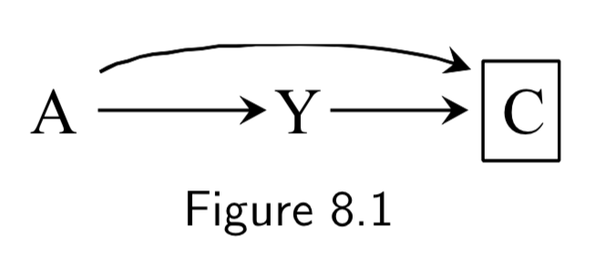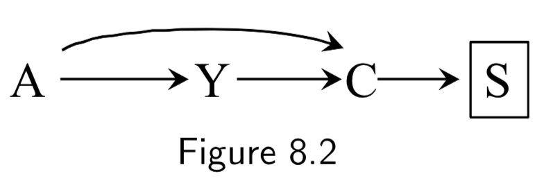
A: Folic Acid supplements Y: Cardiac Malformation C: Death before birth	In this example, we assume folic acid supplements decrease mortality by reducing non-cardiac malformations, cardiac malformatins increase mortality, and cardiac malformations increase mortality. Study restricted participants to fetuses who survived until birth (\(C=0\)). Two sources of association between treatment and outcome: 1. Open path \(A \rightarrow Y\), the causal effect. 2. Open path \(A \rightarrow C \leftarrow Y\) linking \(A\) and \(Y\) due to conditioning on common effect (collider) \(C\). This is the selection bias, specifically, selection bias under the null. The selection bias eliminates ability to make causal inference. If analysis were not conditioned on \(C\), causal inference would be valid.	I.97
A: Folic Acid supplements Y: Cardiac Malformation C: Death before birth S: Parental Grief	This example is the same as the above, except we consider if the researchers instead conditioned on the effect of the collider, namely \(S\), parental grief. This is still selection bias, \(A \rightarrow C \leftarrow Y\) linking \(A\) is open, and association is not causation.	I.98
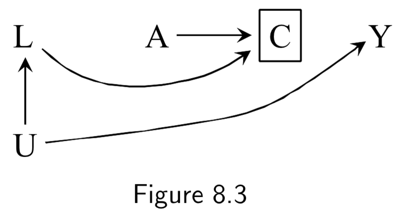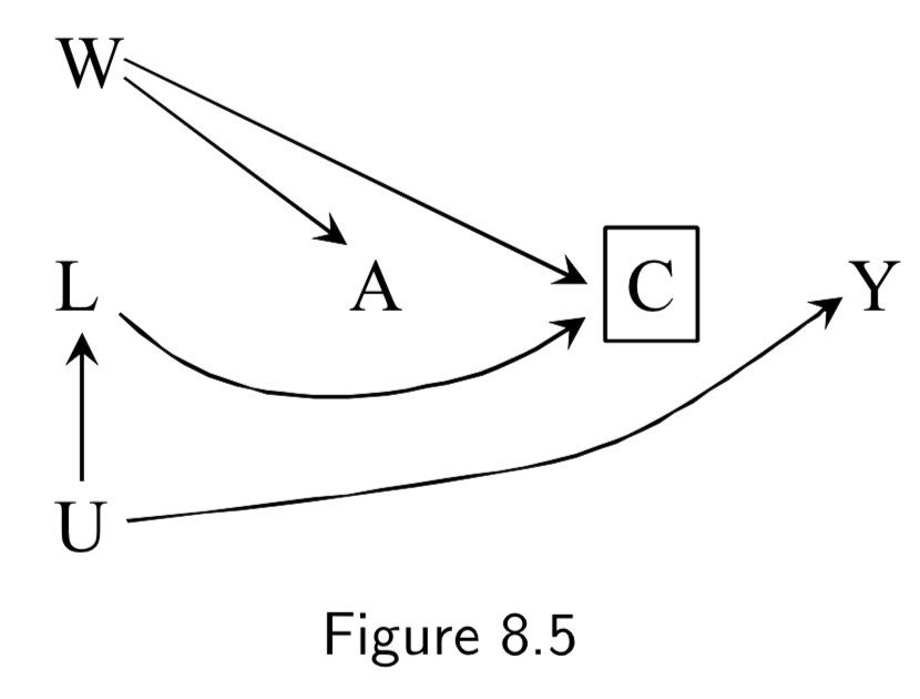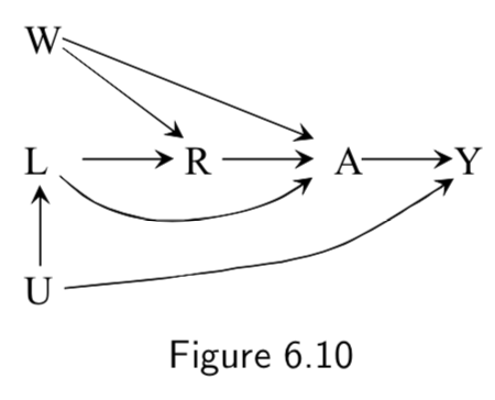
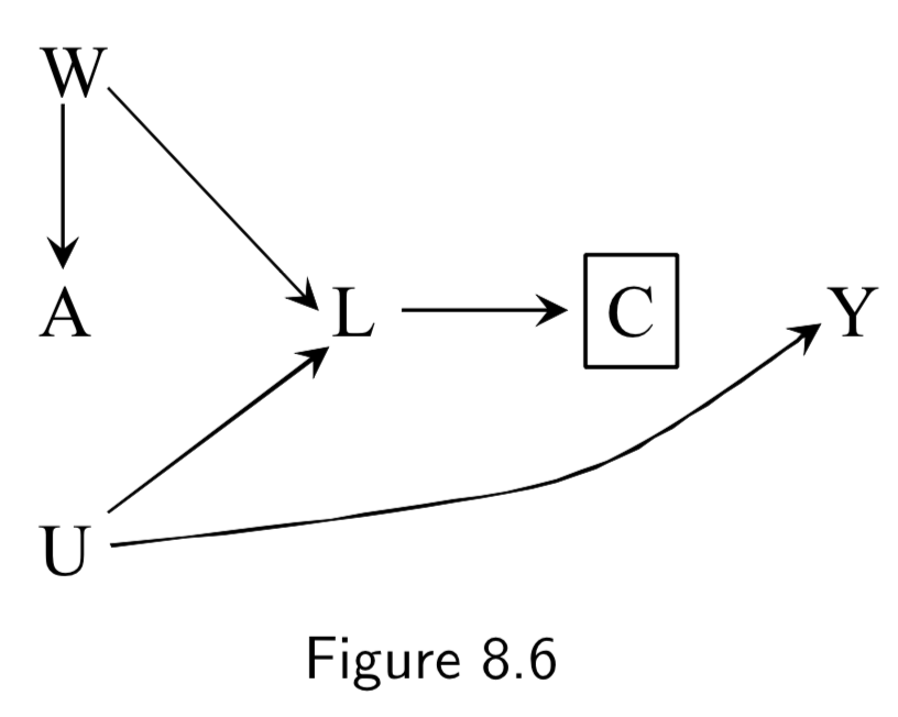
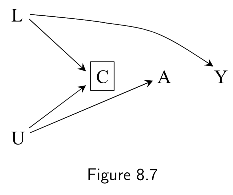
(Note: Missing arrow: \(A \rightarrow Y\) ) A: Antiretroviral treatment Y: 3-year death C: Censoring from study or Missing Data U: High immunosuppresion (unmeasured) L: Symptoms, CD4 count, viral load (unmeasured) ———— W: Lifestyle, personality, educational variables (unmeasured)	Figure 8.3: In this example, individuals with high immunosuppresion – in addition to having higher risk of death – manifest worse physical symptoms that mediates censoring from the study. Treatment also worsens side effects, which increases censoring, as well. \(C\) is conditioned upon, because those are the only ones who actually contribute data to the study. Per d-separation, \(A \rightarrow C \leftarrow L \leftarrow U \rightarrow Y\) is open due to conditioning on \(C\), allowing association to flow from \(A\) to \(Y\) and killing causal inference. Note: This is a transformation of figure 8.1, except instead of \(Y\) acting directly on \(C\), we have \(U\) acting on both \(Y\) and \(C\). Intuition for the bias: if a treated individual with treatment-induced side effects does not drop out (\(C=0\)), this implies that he probably didn’t have high immunosuppresion \(U\), and low immunosuppresion means better outcomes. Hence, there is probably an inverse association between \(A\) and \(U\) among those that don’t drop out. This is an example of selection bias that arises from conditioning on a censoring variable that is a comon effect of both treatment \(A\) and cause \(U\) of the outcome \(Y\). ———— Figure 8.5 is the same idea, except it notes that sometimes additional unmeasured variables may contribute to both treatment and censoring.	I.98
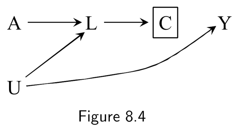(Note: Missing arrow: \(A \rightarrow Y\) ) A: Antiretroviral treatment Y: 3-year death C: Censoring from study or Missing Data U: High immunosuppresion (unmeasured) L: Symptoms, CD4 count, viral load (unmeasured) ———— W: Lifestyle, personality, educational variables (unmeasured)	Same example as 8.3/8.5, except we assume that treatment (especially prior treatment) has direct effect on symptoms \(L\). Restricting to uncensored individuals still implies conditioning on a common effect \(C\) of both \(A\) and \(U\), introducing an association between treatment and outcome. (Note: Unlike in Figure 8.3/8.5, even if we had access to \(L\), stratification is impossible in these DAGs, because while conditioning on \(L\) blocks the backdoor path from \(C\) to \(Y\), it also opens the backdoor path \(A \rightarrow L \leftarrow U \rightarrow Y\) because \(L\) is a collider on that path. IP-weighting, in contrast, could work here. See page I.108 in section 8.5 for a discussion.)	I.98
A: Physical activity Y: Heart Disease C: Becoming a firefighter L: Parental socioeconomic status U: Interest in physical activites (unmeasured)	The goal of this example is to show that while confounding and selection bias are distinct, they can often become functionally the same; this is why some call selection bias “confounding”. Assume that – unknown to the investigators – \(A\) does not cause \(Y\). Parental SES \(L\) affects becoming a firefighter \(C\), and, through childhood diet, heart disease risk \(Y\). But we assume that \(L\) doesn’t affect \(A\). Attraction to physical activity \(U\) affects being physically active \(A\) and being a firefighter \(C\), but not \(Y\). Per these assumptions, there is no confounding, bc no common causes of \(A\) and \(Y\). However, restricting the study to firefighters (\(C=0\)), induces a selection bias that can be eliminated by adjusting for \(L\). Thus, some economists would call \(L\) a “confounder” because adjusting for it eliminates the bias.	I.101
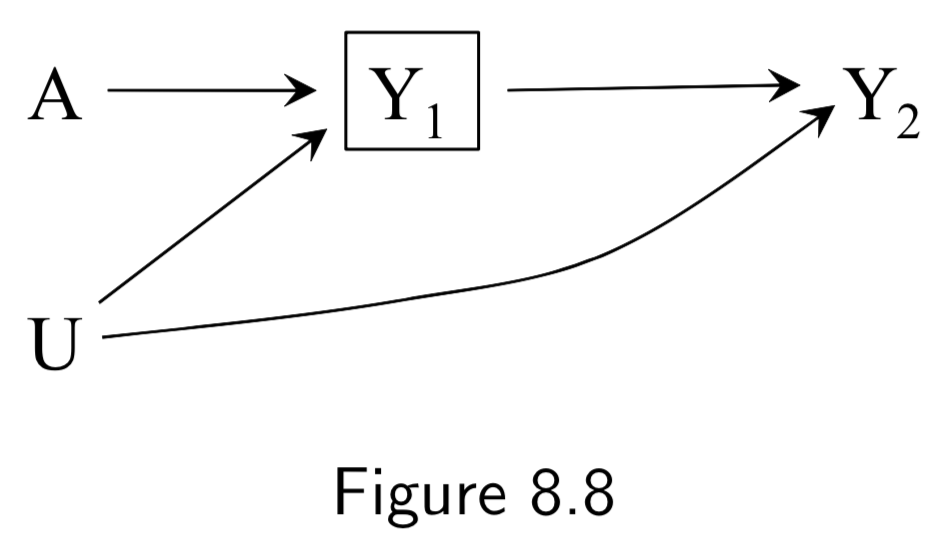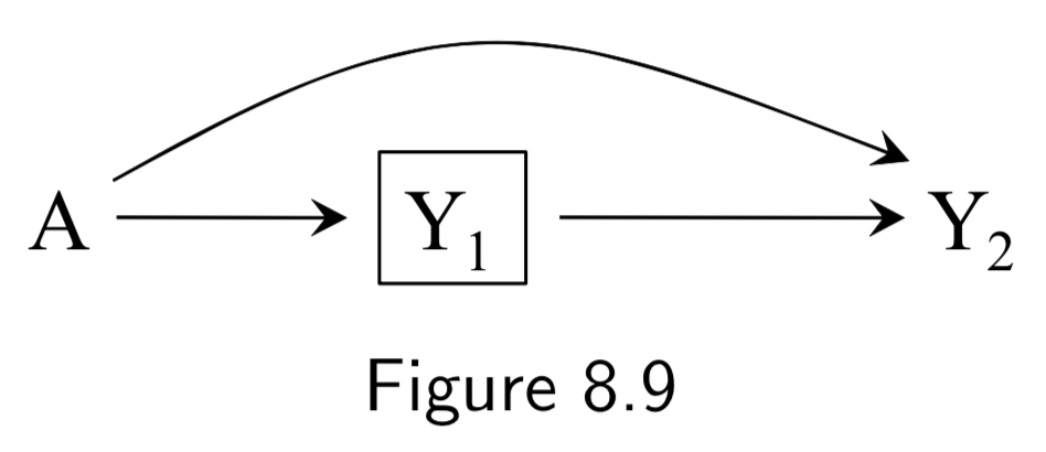A: Heart Transplant Y_1: Death at time point 1 Y_2: Death at time point 2 U: Protective genetic haplotype (unmeasured)	The purpose of this example is to show the potential for selection bias in time-specific hazard ratios. The example depicts a randomized experiment representing the effect of heart transplant on risk of death at two time points, for which we assume the true causal DAG is figure 8.8. In figure 8.8, we assume that \(A\) only directly affects death at the first time point and that \(U\) decreases risk of death at all times but doesn’t affect treatment. In this circumstance, the unconditional associated risk ratios are not confounded. In other words, \(aRR_{AY_1} = \frac{[Y_{1}\|A=1]}{[Y_{1}\|A=0]}\) and \(aRR_{AY_2} = \frac{[Y_{2}\|A=1]}{[Y_{2}\|A=0]}\) are unbiased and valid for causal inference. However, trying to compute time-specific hazard ratios is risky. The process is valid at time point 1 (\(aRR_{AY_1}\) is the same as above), but the hazard ratio at time point 2 is inherently conditional on having survived at time point 1: \(aRR_{AY_2\|Y_{1}=0} = \frac{[Y_{2}\|A=1,Y_{1}=0]}{[Y_{2}\|A=0,Y_{1}=0]}\). Since \(U\) affects survival at time point 1, however, this induces a selection bias that opens a path \(A\rightarrow Y_{1} \leftarrow U \rightarrow Y_{2}\) beteween \(A\) and \(Y_2\). If we could condition on \(U\), then \(aRR_{AY_2\|Y_{1}=0,U}\) would be valid for causal inference. But we can’t, so conditioning on \(Y_{1}=0\) makes the DAG functionally equivalent to Figure 8.9. This issue is relevant to observational and randomized experiments over time.	I.102
(Note: Missing arrow: \(A \rightarrow Y\) ) A: Wasabi consumption (randomized) Y: 1-year death C: Censoring L: Heart Disease U: Atherosclerosis (unmeasured)	This example is of an RCT with censoring. We imagine that there was in reality an equal number of deaths in treatment and control, but there was higher censoring (\(C=1\)) among patients with heart disease and higher censoring among the wasabi arm. As such, we observe more deaths in the wasabi group than in control. Thus, we see a selection bias due to conditioning on common effect \(C\). There are no common causes of \(A\) and \(Y\) – expected in a marginally randomized experiment – so there is no need to adjust for confounding per se. However, there is a common cause \(U\) of both \(C\) and \(Y\), inducing a backdoor path \(C \leftarrow L \leftarrow U \rightarrow Y\). As such, conditioning on non-censored patients \(C=0\) means we have a selection bias that turns \(U\) functionally into a confounder. \(U\) is unmeasured, but the backdoor criterion says that adjusting for \(L\) here blocks the backdoor path. The takeaway here is that censoring or other selection changes the causal question, and turns the counterfactual outcome into \(Y^{a=1,c=0}\) – the outcome of receiving the treatment and being uncensored. The relevant causal risk ratio, for example, is thus now \(\frac{E[Y^{a=1,c=0}]}{E[Y^{a=0,c=0}]}\) – “the risk if everyone had been treated and was uncensored” vs “the risk if everyone were untreated and remained uncensored.” In this sense, censoring is another treatment.	I.105
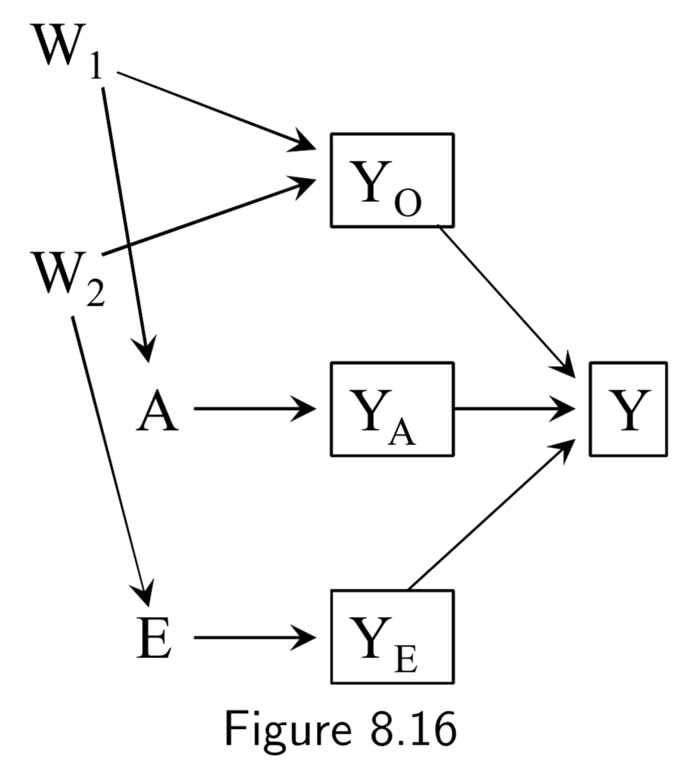
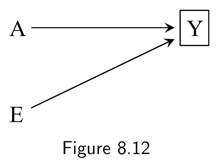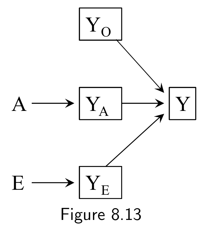A: Surgery Y: Death E: Genetic hapltype ———— Death subsplit by causes: (not recorded) Y_A: Death from tumor Y_E: Death from heart attack Y_A: Death from other causes	In this example, Figure 8.12, surgery \(A\) and haplotype \(E\) are: (i) marginally independent (i.e. haplotype doesn’t affect probability of receiving surgery), and (ii) associated conditionally on \(Y\) (i.e. probability of receiving surgery does vary by haplotype within at least one stratum of the haplotype). The purpose of this example is to show that despite this fact, situations exist in which \(A\) and \(E\) remain conditionally independent within some haplotypes. Key idea here is that to recognize that if you split death into different causes (even if this isn’t recorded), \(A\) and \(E\) affect different sub-causes in different ways (specifically, \(A\) removes tumor, and \(E\) prevents heart attack). Arrows from \(Y_{A}\), \(Y_{E}\), and \(Y_{O}\) to \(Y\) are deterministic, and \(Y=0\) if and only if \(Y_{A} = Y_{E}=Y_{O}=0\), so conditioning on \(Y_{0}=0\) implicitly conditions the other \(Y\)s to zero. This also blocks the path between \(A\) and \(E\), since it is conditioning on non-colliders \(Y_{A}\), \(Y_{E}\), and \(Y_{O}\). In contrast, conditioning on \(Y=1\) is compatible with any combination of \(Y_{A}\), \(Y_{E}\), and \(Y_{O}\) being equal to 1, so the path between \(A\) and \(E\) is not blocked. The ability to break the conditional probability of survival down in this way is an example of a multiplicative survival model.	I.105
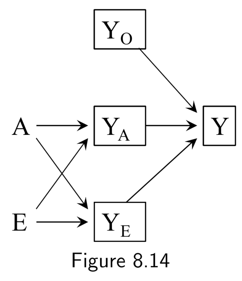A: Surgery Y: Death E: Genetic hapltype ———— Death subsplit by causes: (not recorded) Y_A: Death from tumor Y_E: Death from heart attack Y_A: Death from other causes	Same setup as in the examples of Figure 8.12 and 8.13. However, in all of these DAGs, \(A\) and \(E\) affect survival thrugh a common mechanism, either directly or indirectly. In such cases, \(A\) and \(E\) are dependent in both strata of \(Y\). Taken together with the example above, the point is that *conditioning on a collider always* induces an association between its causes, but that this association may or may not be restricted to certain levels of the common effect**.	I.105

Some additional (but structurally redundant) examples of selection bias from chapter 8:

Example	Notes	Page
(Note: Missing arrow: \(A \rightarrow Y\) ) A: Occupational exposure Y: Mortality C: Being at Work U: True health status L: Blood tests and physical exam ———— W: Exposed jobs are eliminated and workers laid off	(Note: DAGS 8.3/8.5 work just as well, here.) Healthy worker bias: If we restrict a factory cohort study to those individuals who are actually at work, we miss out on the people that are not working due to either: (a) disability caused by exposure, or (b) a common cause of not working and not being exposed.	I.99
(Note: Missing arrow: \(A \rightarrow Y\) ) A: Smoking status Y: Coronary heart disease C: Consent to participate U: Family history L: Heart disease awareness ———— W: Lifestyle	(Note: DAGS 8.4/8.6 work just as well, here.) Self-selection bias or Volunteer bias: Under any of the above structures, if the study is restricted to people who volunteer or choose to participate, this can induce a selection bias.	I.100
(Note: Missing arrow: \(A \rightarrow Y\) ) A: Smoking status Y: Coronary heart disease C: Consent to participate U: Family history L: Heart disease awareness ———— W: Lifestyle	(Note: DAGS 8.4/8.6 work just as well, here.) Selection affected by treatment received before study entry: Generalization of self-selection bias. Under any of the above structures, if the treatment takes place before the study selection or includes a pre-study component, a selection bias can arise. Particularly high-risk in studies that look at lifetime exposure to something in middle-aged volunteers. Similar issues often arise with confounding if confounders are only measured during the study.	I.100

Measurement Bias (Chapter 9)

Example	Notes	Page
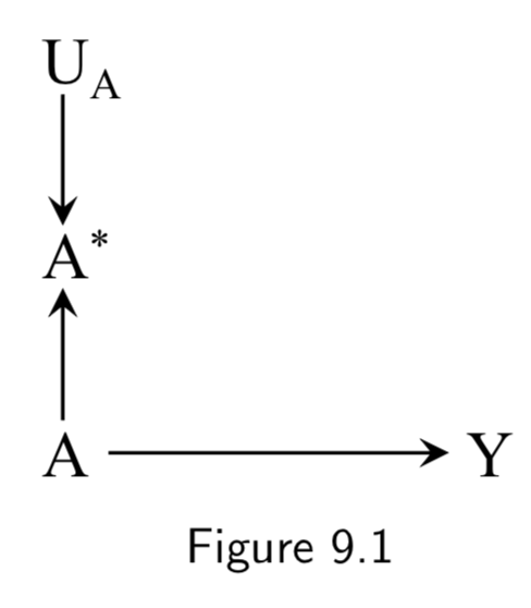A: True Treatment A: Measured treatment Y: True Outcome U_A*: Measurement error	This DAG is simply to demonstrate how the measured treatment \(A^{}\) (aka “measure” or “indicator”) recorded in the study is different from the true* treatment (aka “construct”). It also introduces \(U_{A}\), the measurement error variable, which encodes all the factors other than \(A\) that determine \(A^{}\) Note: \(U_{A}\) and \(A^{}\) were unnecessary in discussions of confounding or selection bias because they are not a part of a backdoor path and no variables are conditioned on them.	I.111
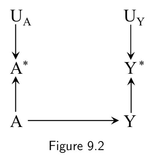A: True Treatment A: Measured treatment Y: True Outcome Y: Measured outcome U_A: Measurement error for A U_Y: Measurement error for Y	This DAG adds in the notion of imperfect measurement for the outcome as well as the treatment. Note that there is still no confounding or selection bias at play here, so measurement bias or information bias is the only thing that would break the link between association and causation. Figure 9.2 is an example of a DAG with independent nondifferential error.	I.112
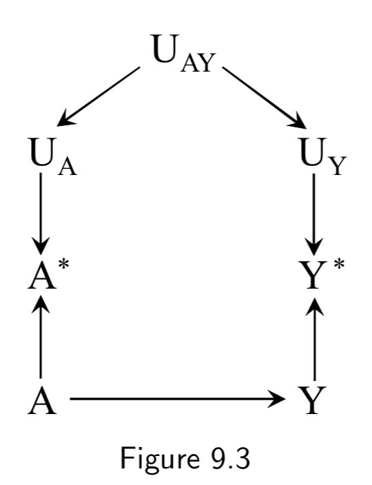A: Drug use A: Recorded history of drug use Y: Liver toxicity Y: Liver lab values U_A: Measurement error for A U_Y: Measurement error for Y U_AY: Measurement error affecting A and Y (e.g memory and language gaps during interview)	In Figure 9.2 above, \(U_{A}\) and \(U_{Y}\) are independent according to d-separation, because the path between them is blocked by colliders. Independent errors could include EHR data entry errors that occur by chance, technical errors at a lab, etc. In this figure, we add \(U_{AY}\) to note the existence of dependent errors. For example, communication errors that take place during an interview with a patient could effect both recorded drug use and previous recorded lab tests. Figure 9.3 is an example of dependent nondifferential error.	I.112
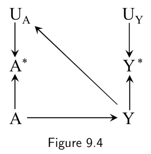
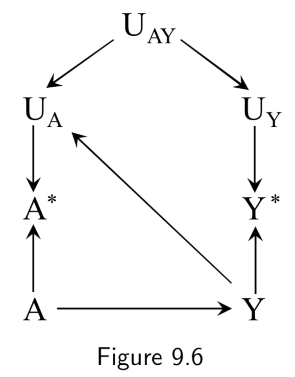
A: Drug use A: History of drug use per patient interview Y: Dementia Y: Dementia diagnosis U_A: Measurement error for A U_Y: Measurement error for Y ____ __U_AY: Measurement error affecting A and Y	Recall bias is one example of how the true outcome can bias treatment measurement error. In this example, patients with dementia are less able to effectively communicate, so true cases of the disease are more likely to have faulty medical histories. Another example of recall bias could be in a study of the effect of alcohol use during pregancy \(A\) on birth defects \(Y\), if the alcohol intake is measured by recall after delivery. Bad medical outcomes, especially ones like complicated births, often affect patient recall and patient reporting. Figure 9.4 is an example of independent differential measurement error. Adding dependent errors such as a faulty interview makes Figure 9.6 an example of dependent differential error.	I.113
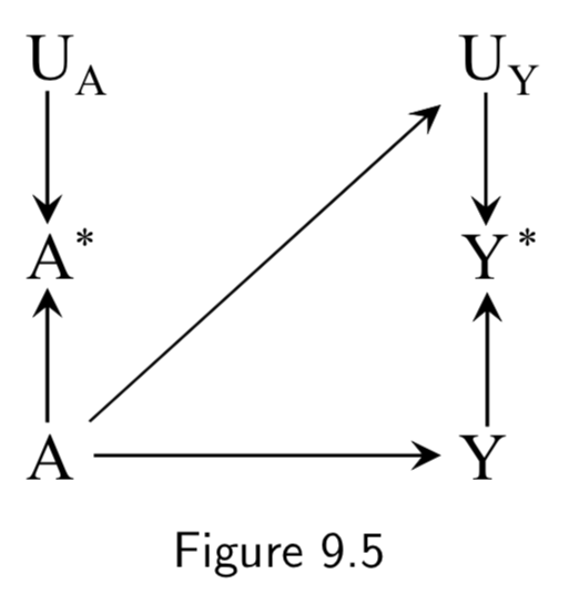
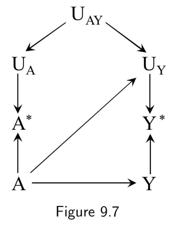
A: Drug use A: Recorded history of drug use Y: Liver toxicity Y: Liver lab values U_A: Measurement error for A U_Y: Measurement error for Y ____ __U_AY: Measurement error affecting A and Y	An example of true treatment affecting the measurement error of the outcome could also arise in the setting of drug use and liver toxicity. For example, if a doctor finds out a patient has a drug problem, he may start monitoring the patients liver more frequently, and become more likely to catch aberrant liver lab values and record them in the EHR. Figure 9.5 is an example of independent differential measurement error. Adding dependent errors such as a faulty interview makes Figure 9.7 an example of dependent differential error.	I.113
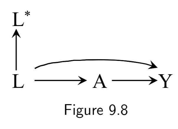A: Drug use Y: Liver toxicity L: History of hepatitis L*: Measured history of hepatitis	This example demonstrates mismeasured confounders. Controlling for \(L\) in Figure 9.8 would be sufficient to allow for causal inference. However, if \(L\) is imperfectly measured – say, because it was retrospectively recorded from memory – then the standardized or IP-weighted risk ratio based on \(L^{}\) will generally differ from the true causal risk ratio. A cool observation is that since noisy measurement of confounding can be thought of as unmeasured confounding, Figure 9.9 is actually equivalent to Figure 7.5: \(L^{}\) is essentially a surrogate confounder (like Figure 7.5’s \(L\)) for an unmeasured actual confounder (Figure 7.5’s \(U\) playing the role of Figure 9.9’s \(L\)). Hence, controlling for \(L^{*}\) will be better than nothing but still flawed.	I.114
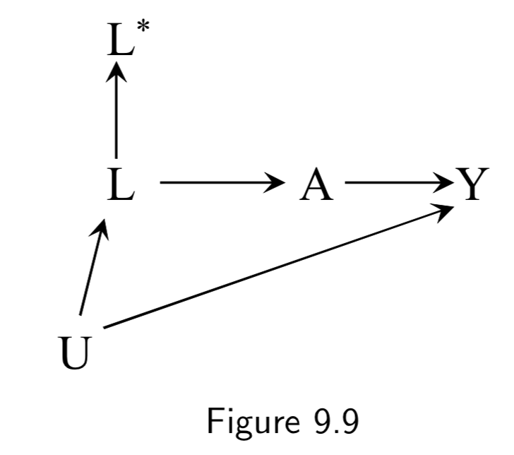A: Aspirin Y: Stroke L: Heart Disease U: Atherosclerosis (unmeasured) L*: Measured history of heart disease	Figure 9.9 is the same idea as Figure 9.8: Even though controlling for \(L\) would be sufficient, a mismatched \(L^{}\) is insufficient to block the backdoor path in general. Another note here is that mismeasurement of confounders can result in apparent effect modification. For example, if all participants who reported a history of heart disease (\(L^{}=1\)) and half the participants who reported no such history (\(L^{}=0\)) actually had heart disease, then stratifying on (\(L^{}=1\)) would eliminate all confounding in that stratum, but statifying on (\(L^{}=0\)) would fail to do so. Thus one could detect a spurious assocation in (\(L^{}=0\)) but not in (\(L^{}=1\)) and falsely conclude that \(L^{}\) is an effect modifier. (See discussion on I.115.)	I.114
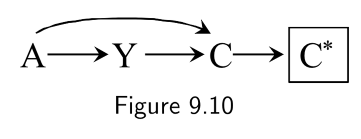A: Folic Acid supplements Y: Cardiac Malformation C: Death before birth C*: Death records	Conditioning on a mismeasured collider induces a selection bias, because \(C^{*}\) is a common effect of treatment \(A\) and outcome \(Y\).	I.115
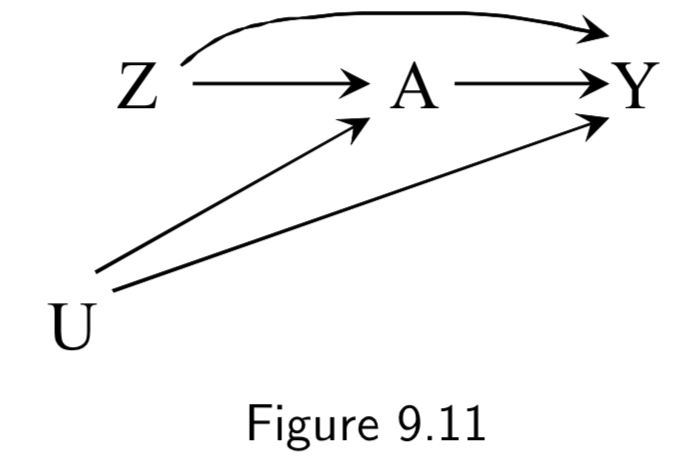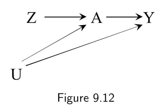Z: Assigned treatment A: Heart Transplant Y: 5-year Mortality (Ignore U here)	Figure 9.11 is an example of an intention-to-treat RCT. ITT RCT’s can be almost thought of as an RCT with a potentially misclassified treatment. However, unlike a misclassifed treatment, the treatment assignment \(Z\) has a causal effect on the outcome \(Y\), both (a) by influencing the actual treatment \(A\), and (b) by influencing study participants who know what \(Z\) is and change their behavior accordingly. Hence, the causal effect of \(Z\) on \(Y\) depends on the strength of the arrow \(Z \rightarrow Y\), the arrow \(Z \rightarrow A\), and the arrow \(A \rightarrow Y\). Double-blinding attempts to remove \(Z \rightarrow Y\) (Figure 9.12).	I.115
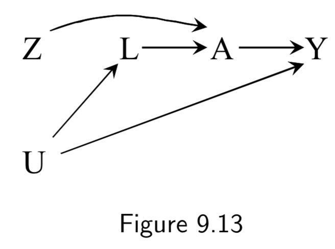
Z: Assigned treatment A: Heart Transplant Y: 5-year Mortality U: Illness Severity (unmeasured)	By including \(U\), we are considering the fact that in an IIT study, severe illness (or other variables) contribute to some patients to seek out different treatment than they’ve been assigned. Note that there is a backdoor path \(A \leftarrow U \rightarrow Y\) and thus confounding for the effect of \(A\) on \(Y\), requiring adjustment. However, there is no confounding of \(Z\) and \(Y\), and thus no need for adjustment. This explains why the intention-to-treat effect is often estimated in lieu of the per-protocol effect. Taken together, per-protocol effect brings with it unmeasured confounding, and IIT brings risk of misclassification bias. So one needs to trade these off when deciding which to use. (Full discussion below and on I.120)	I.115
Z: Assigned treatment A: Heart Transplant Y: 5-year Mortality U: Illness Severity (unmeasured) L: Measured factors that mediate U	This example is of a as-treated analysis, a type of per-protocol analysis As-treated includes all patients and compares those treated (\(A=1\)) vs not treated (\(A=0\)), independent of their assignment \(Z\). As-treated analyses are confounded by \(U\), and thus depend entirely on whether they can accurately adjust for measurable factors \(L\) to block the backdoor paths between \(A\) and \(Y\).	I.118
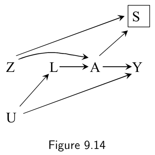Z: Assigned treatment A: Heart Transplant Y: 5-year Mortality U: Illness Severity (unmeasured) L: Measured factors that mediate U S: Selection filter (A=Z)	This example is of a conventional per-protocol analysis, a second method to measure per-protocol effect. Conventional per-protocol analyses limit the population to those who adhered to the study protocol, subsetting to those for whom \(A=Z\). This method induces a selection bias on \(A=Z\), and thus still requires adjustment on \(L\).	I.118

Some additional (but structurally redundant) examples of measurement bias from chapter 9:

DAG	Example	Notes	Page
	A: Drug use A: Recorded history of drug use Y: Liver toxicity Y: Liver lab values U_A: Measurement error for A U_Y: Measurement error for Y	Reverse causation bias is another example of how the true outcome can bias treatment measurement error. In this example, liver toxicity worsens clearance of drugs from the body, which could affect blood levels of the drugs.	I.112